| 1. What
does it do ?
This module calculates and displays
radix-2 FFT and IFFT for a complex finite duration sequence with sequence
length upto 256 points.The real and imaginary part sequences can be generated
in four ways - by loading them from preloaded example files , by opening
a previously stored project file , by editing interactively in the main
window itself and by invoking the sequence generation module from File
menu.
The sequence can be saved into *.prj
file in the default project directory. The FFT and IFFT output sequences
also can be stored in *.txt file and the plots can be saved in *.ps (Postscript
Format) files in the default project directory.
The program allows various options to
display the FFT in polar or rectangular form in drop line or curve modes.
2. Main
Window Components

2.1 'Data Points' Pulldown Box
This is a Browse Entry Box. When
an example file or project file is opened the length of the sequences (both
sequences are assumed to be of same length everywhere in this program)
will appear in this box. User can choose an entry here by pulling down
the entry box.This will result in resetting all the plots and pushing all
powers of 2 upto 256 and above the selected value into the DFT Points box.
2.2 'DFT Points' Pulldown Box
This will contain the choices for
the number of DFT points that should be calculated when FFT of real part
or imaginary part or the complex sequence is carried out. The value here
gets automatically set at the sequence length and can only be increased
by making another choice.
2.3 The 'Index for Input' Box
This box entry decides the index
of real and imaginary part sequences open for editing currently. and the
value that is desired at that value of index.This pulldown box will contain
choices depending on the choice made in the 'Data Points' box above.The
result of choices made will be visible immediately in the plot which appears
in the first plot area in the first row.
2.4 The 'Real Part' and 'Imag.
Part' Boxes
These box entries decide the values
that are desired at the value of index chosen in the above box.The result
of choices made will be visible immediately in the plots which appears
in the first and second plot areas in the first row.
2.5 The 'Reset' Buttons
Clean reset the two sequences to
'empty' and reset the 'Data Points' number to zero.
3. Menubar
Items
3.1 File Menu
3.1.1 Load
Example
-Choose and load one of the 10 example
sequence pairs included in the program.
3.1.2 Load
Project
Load a sequence pair by opening a
*.prj file saved in an earlier session.The default directory will be '/Projects/fft'
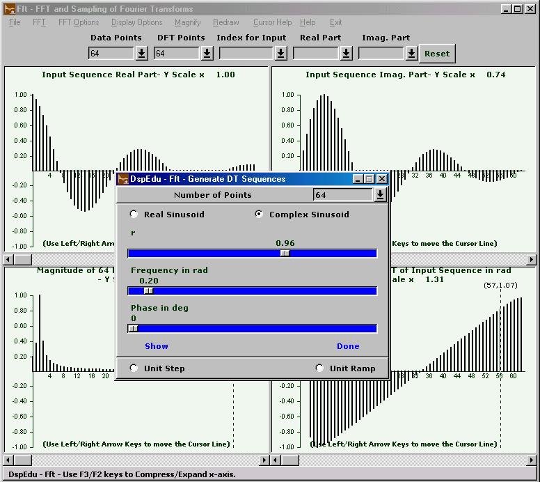
3.1.3 Generate
DT Sequences
Brings up a new window with options
to generate and set real part and imaginary part to sinusoidal,step and
ramp sequences.The frequency ,phase and decrement of damped sinusoids can
be chosen by using a pair of slider controls which appear in that window.The
sequences can be examined and edited before final acceptance.The sequence
length can be between 8 and 256.
3.1.4 Save
Project
-Brings up a standard Windows Save
Dialog box which opens into '/Projects/fft' by default and shows *.prj
as the default extension.The number of points in the sequences and sequence
data will be stored as an ascii file with selected name and 'prj' extension.The
program assumes write permission in the chosen directory , overwrites with
prompt and does not provide confirmation dialog.
3.1.5 Save
FFT Output
Brings up a standard Windows Save
Dialog box which opens into '/Projects/fft' by default and shows *.txt
as the default extension. The number of points in the sequences, the sequence
data , FFT output data etc.will be stored as an ascii file with selected
name and 'txt' extension. The number of points calculated in FFT will be
as per the current values in 'DFT Points' box or 512 if 'Fourier Transform'
option is selected. The program assumes write permission in the chosen
directory , overwrites with prompt and does not provide confirmation dialog.
3.1.6 Save
Plots
Brings up a standard Windows Save
Dialog box which opens into '/Projects/fft' by default and shows *.ps as
the default extension.The four plots which currently appear in the four
plot areas will be saved as four postscript files with selected names and
'ps' extension. The number of points calculated in FFT will be as per the
current values in 'DFT Points' box . The program assumes write permission
in the chosen directory , overwrites with prompt and does not provide confirmation
dialog.
3.2 FFT Menu
3.2.1 Show
FFT
Carries out the FFT Computation
for the Complex Sequence and plots the result in first and second plot
areas in the second row. The number of DFT Coefficients calculated will
be as per the current entry in the DFT Points box. Magnitude and Angle
are plotted by default. Option to plot the real part and imaginary part
is available under the Options menu.
3.2.2 Show
FFT of Real Part
Carries out the FFT Computation
for the Real Part Sequence and plots the result in first and second plot
areas in the second row. The number of DFT Coefficients calculated will
be as per the current entry in the DFT Points box. Magnitude and Angle
are plotted by default. Option to plot the real part and imaginary part
is available under the Options menu.
3.2.3 Show
FFT of Imag. Part
Carries out the FFT Computation
for the Imaginary Part Sequence and plots the result in first and second
plot areas in the second row. The number of DFT Coefficients calculated
will be as per the current entry in the DFT Points box. Magnitude and Angle
are plotted by default. Option to plot the real part and imaginary part
is available under the Options menu.
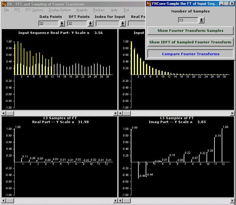
3.2.4 Sample
FT of Input Sequence
Brings up a new window. This menu
options allows the user to calculate and display a certain number of samples
of Fourier Transform of the Complex Input Sequence which are evenly spaced
in the Unit Circle in z-domain. The number of samples to be calculated
can be chosen by pulling down an entry box in the new window. The calculated
samples will be displayed in the first and second plot areas in the second
row (magnitude and angle in the default case).
Inverse DFT of these samples can
be calculated and they will be shown along with the original values of
real part and imaginary part of the input sequence using a different color
for the sake of comparison.
The third command button in the
new window allows the user to calculate the Fourier Transforms of the original
input sequence and the sequence obtained by Inverse DFT on the samples
of Fourier Transform.
These Fourier Transforms are calculated
by 512-Point FFT and curve-mode two-sided display. The two Fourier Transforms
calculated will be displayed in the first and second plot areas in the
second row using different colors for the sake of comparison.
3.2.5 Show
IFFT of Input Sequence
In this case , the real and imaginary
part input sequences are taken to be real part and imaginary part of DFT
of some time-domain sequence and that sequence is calculated by IFFT. The
calculation results are displayed in the second row.

3.3 FFT Options
3.3.1 FFT Options
Show Fourier Transform - Calculate
the 512-Point FFT (disregarding the entry in 'DFT Points' box) and display
a two-sided plot by joining the points by stright-line interpolation.
Show DFT Coefficients - Calculate
FFT as per the entry in 'DFT Points' box and display as per current display
option. This is the default option.
Rectangular Form - Show DFT
Coefficients or Fourier Transform in Rectangular Form.
Polar Form - Show DFT Coefficients
or Fourier Transform in Polar Form. This is the default.
3.3.2 Numeric
Result Windows Enable/Disable
Enabling will result in a window
containing the convolution results popping up after every FFT computation.
Default - Disable
3.3 Display Options
3.4.1 Display
Mode
Data Points - The plots will be
line plots , a line representing the data value.
Data Envelope - A piece-wise linear
curve joining the data points will be shown. Changing this option comes
into effect immediately in the existing plots.
3.4.2 Display
Color Options
Normal Plot Color - The color used
to draw x1(n) , x2(n) and convolution outputs.
Second Plot Color - The color used
to draw a second plot in the same plot area.
Background Color - The color used
as background for all the four plot areas. These three options bring up
standard windows color selection dialog and changes take immediate effect
Schemes - Three color schemes in
addition to default scheme are provided.Changes take immediate effect.
3.5 Magnify
Magnify the x-axis by various fixed
factors. F2 key will expand the x-axis and F3 key will compress it.However
this menu provides fixed scale factors for convenience.
3.6 Redraw
Re-scale all the four plot areas
and redraw all the plots - needed after a resize of the main window.
3.7 Help
-This page.
3.8 Exit
4. Restrictions
in the Evaluation Version
The Module can be run only 15 times and each session will last only for 10 minutes.
There are no feature limits.
5. Author
Suresh Kumar K.S
Department of Electrical Engineering
National Institute of Technology,Calicut-673601,Kerala,India
sureshks (at) nitc (dot) ac (dot) in
29th April 2004
|

